DATA/ AURA/ OMO3PR
OMO3PR README File
J.F. de Haan and J.P. Veefkind, KNMI
Last update: January 24, 2008
Release: Provisional
Overview
This document provides a brief description of the OMO3PR data
product. OMO3PR contains the retrieved ozone profile and the
corresponding a-priori ozone profile, error covariance matrix
and averaging kernel. Further it contains ancillary
information produced by the optimal estimation algorithm
applied to OMI global mode measurements. An OMO3PR data file
contains the measurements of the sunlit part of a single orbit, from
the South to the North pole. The OMI swath width is approximately 2600
km.
The ozone profile is given in terms of the layer-columns of
ozone in DU for an 18-layer atmosphere. The layers are
nominally bounded by the pressure levels: [ surface pressure, 700, 500, 300,
200, 150, 100, 70, 50, 30, 20, 10, 7, 5, 3, 2, 1, 0.5, and
0.3 hPa.
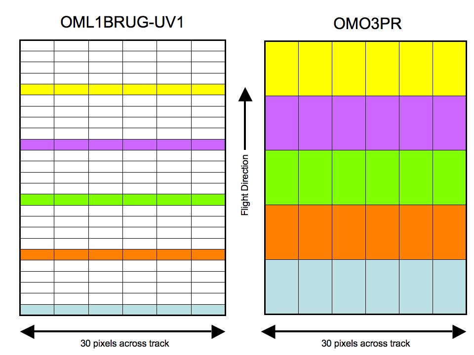
In view of the calculation times involved about 20% of the
pixels are processed. As shown in Figure 1, four out of five
measurements in the flight direction are skipped.
Figure 1. Schematic
showing the sampling of the OML1BRUG UV1 data by the OMO3PR algorithm.
In the flight direction OMO3PR processes one row of groundpixels and
skips the next four. In the across track direction all 30 groundpixels
are processed. The colors indicate the same rows for OML1BRUG and
OMO3PR, white rows are skipped by OMO3PR.
The ozone profile listed in the output file is in DU per
layer. This can easily be converted to an average volume
mixing ratio per layer using
<vmr>i = 1.2672 Ni / DPi
with Ni the layer-column in DU, DPi the pressure
difference between the top and bottom of the layer in hPa and
<vmr>I the average volume mixing ratio in ppmv.
You may refer to OMI Level 2 Ozone Profile
Data Product Specification for release specific information and details about software versions.
Please find other information on OMO3PR at http://www.knmi.nl/omi/research/product/Ozone/omproo3.html.
Go to the OMO3PR L2 dataset directory
Go to the OMO3PR station overpass data directory
Algorithm Description
The retrieval algorithm is based on optimal estimation
(Rodgers, 2000) with climatological a-priori information.
Basically the amount of ozone in each atmospheric layer is
adjusted such that the difference between the modeled and
measured sun-normalized radiance is minimal. As the
information content in the measured spectrum is not large enough to
determine the ozone amount for all layers, a side-constraint
is used by demanding that the retrieved profile does not
differ too much from the climatological average. The
measurements are taken from the UV1 channel (270 nm –
310 nm) and the first part of the UV2 channel (310 nm
– 330 nm). Here two UV2 pixels are combined to
obtain the spectrum of a pixel that corresponds to a pixel in
the UV1 channel. Small differences in alignment are dealt with
by assuming that the cloud cover and the surface albedo for
the two channels can be different.
The algorithm uses the newly developed LABOS radiative
transfer model, which replaces the 6 stream Lidort-a model
that is currently used for GOME and GOME 2. LABOS includes an approximate treatment of rotational
Raman scattering, pseudo spherical correction for direct
sunlight, and corrections for the initial assumption that the
atmospheric layers are homogeneous. Polarization is ignored
in the RTM calculations and a LUT with polarization correction factors is used to compensate for this. Forward calculations
are performed in the wavelength range 267 – 332 nm
on a sufficiently fine grid such that after interpolation the
error in the reflectance is less than about 0.2% for any
wavelength considered. This facilitates convolutions with rotational Raman lines and convolutions with the OMI slit function
after multiplication with a high-resolution solar spectrum. A
Chebyshev expansion combined with a LUT is used to perform the
convolution with the OMI slit function in an efficient manner.
The surface below the atmosphere is Lambertian and has an initial value taken from a surface albedo climatology. The
surface albedo for the UV1 and UV2 channels are fitted separately.
The measurement errors used in optimal estimation are taken
from the level 1b product. Currently, the Fortuin-Kelder
climatology is used as a-priori, but it may be replaced by a
different climatology in the near future. Optimal estimation
is started with the a-priori and a maximum of 7 iteration
steps is allowed for convergence. The current default is that
the convergence of the state vector is tested according to
Eq. (5.28) in Rogers (2000), with a threshold of 1.0.
Data Quality Assessment
- Synthetic Data
The profile algorithm was applied to synthetic data produced
by a radiative transfer code and it results were compared
with the ozone profile used to simulate the measured spectrum
and with the results obtained from a prototype retrieval code
that has been developed for GOME2. These tests gave good results.
- Comparisons with Correlative Data
When applied to OMI measured data convergence is often good
(above snow/ice there are problems). Limited comparisons with
MLS, GOMOS and sonde measurements show in general good results. Figure 2 shows an example of
compasrisons with MLS for August 1, 2007.
Figure 2. Comprison
for OMI and MLS ozone profiles on August 1, 2007, for the latitude
range between 60 and 90 N. The left plot shows the average ozone
profiles for 861 comparisons. The MLS profiles are in black and the OMI
profiles in red, the error bars indicate the standard deviation. The
right plot shows the difference in percent between OMI and MLS. The
black curve shows the mean difference, the red curve shows the absolute
difference o OMI-MLS.

- Performance for Ozone Hole Conditions
There are some indications
that the retrieved profile above the ozone maximum follows the
a-priori profile too closely. Also, for ozone hole conditions the
algorithm may not converge. It may be necessary to change
the a-priori covariance matrix to remedy this.
Product Description
The OMO3PR product is written as an HDF-EOS5 swath file. For
a list of tools that read HDF-EOS5 data files, please visit
this link: http://disc.gsfc.nasa.gov/Aura/tools.shtml.
The main parameters listed in the output product are: ozone
profile, ozone profile error covariance matrix, ozone
a-priori profile, ozone a-priori error covariance matrix,
ozone averaging kernel, number of iterations, pressure
levels for the layers, latitude, longitude, viewing direction and solar position.
A single file contains approximately 330 OMI measurements of 30 ground
pixels each. Thus the data fields have a dimensions of approximately
330 in the flight direction, 30 in the across track direction and 18
pressure levels.
In order to reduce the file size some data is written as
integer. Scaling information is provided by the attributes
(part of properties) of a certain output field. The overall
settings for the processing can be found under CAS
‘Additional’,
‘FILE_ATTRIBUTES’, and the attributes of
the properties. There the OPF (operational parameter file) settings
are listed.
Data Availability
Full OMO3PR data, as well as subsets of these data over many ground stations and along Aura validation aircraft flights paths are available through the Aura Validation Data Center (AVDC) website to those investigators who are associated with the various Aura science teams. Christian Retscher is the point of contact at the AVDC.
Contact Information
Questions related to the OMO3PR dataset should be directed to the Principal Investigator. For questions and comments related to the OMO3PR algorithm and data quality please send mail to contact Mark Kroon (KNMI).
Go to the OMO3PR L2 dataset directory
Go to the OMO3PR station overpass data directory
|

